Reinforcement Learning (Part 5) - Q Learning and Optimal Policy Finding

This is the 5th part of the Reinforcement Learning Series: Here I discuss about techniques to finding optimal policies, and then demonstrate the popular Q-learning algorithm.

Introduction

In my previous post, we learned how we can use different algorithms to estimate the value function of a Markov decision process. If you are unfamiliar with these concepts/terminologies, I recommend checking out my last post before starting.

In this post, we shall finally take a look at how we can use the value estimates to know which actions to take, and how we can find out optimal policies in a reinforcement learning system.

So far, we have seen that given a policy 𝜋, it is possible to use different kinds of algorithms to get an estimate of the value function of the policy 𝜋, which will tell us how valuable each state is. We learned about the following methods:

1. Dynamic Programming with Bellman equation.

2. Monte Carlo algorithm.

3. Temporal Different learning algorithms.

We applied all of these methods for our maze game and estimated the value function under the policy of random movement (i.e., all four directions are picked with equal probability). Also, I have indicated before that at every state, if we just keep taking some action that improves the value of the state, we can reach the end goal for this scenario. However, in general, this procedure can get stuck in a local optimum. Imagine that you have estimates on how much traffic will be on different roads while commuting to your work, so you accordingly choose a particular road. But maybe, there is some construction work going on that road, due to which the best possible road that you have in mind is actually sub-optimal.

Optimal Policy Finding

However, to find an optimal policy, we can follow this principle and try to estimate the Q-function (quality function) instead of the value function for every state-action pair. That means,

1. For dynamic programming, you can use the Bellman equation of expressing Q(s, a) as a sum over its next state-action Q-values.

2. For Monte Carlo algorithms, we keep track of rewards and gains grouped by the state-action pairs instead of grouping by states only.

3. For temporal difference algorithms, we update Q(s, a) as

\(Q^\pi_{new}(S_t, A_t) = Q^\pi_{old}(S_t, A_t) + \alpha \left( R_{t+1}(A_t) + \gamma \sum_{a \in A} \pi(a \mid S_{t+1}) Q^\pi_{old}(S_{t+1}, A_{t+1} = a) - Q^\pi_{old}(S_t, A_t) \right)\)

which is very similar to the TD iteration rule that we have seen before.

So, let’s say for a policy 𝜋, we have an estimate of Q-value function Q𝜋(s, a). Then, based on the above principle, we can choose the action a which has the highest Q-value given state “s”. In particular,

\(\pi_{new}(a \mid s) = \begin{cases} 1 & \text{ if } a = \arg\max_{a \in A} Q^\pi(s, a)\\ 0 & \text{ otherwise} \end{cases} \)

Naturally, this new policy 𝜋_{new} is called greedy with respect to the Q-function. Since 𝜋_{new} is a new policy, the Q-function for this new policy will also change. Using the learning techniques, we can obtain its Q-function estimate, and then again from that Q-function, we can take the greedy approach. We can repeat these two steps Policy Evaluation (Q-function estimation) and Policy Improvement (Improving the policy by taking greedy action with respect to the current Q-function estimate), until we reach a halt. At that time, we have found a policy that is performing best according to its own value function, and hence it cannot be improved further. Thus, it becomes an optimal policy.

This approach to finding the optimal policy is called Policy iteration.

Q-Learning

Q-learning is a fundamental reinforcement learning algorithm that plays a pivotal role in finding optimal policies for Markov decision processes (MDPs). It's a powerful and widely used technique because it combines the benefits of both model-free and off-policy learning. Now, before delving further, let us understand these two key terms: model-free and off-policy learning.

• Model Free: It is basically some kind of learning algorithm that can accumulate experience and use that to estimate the value, as opposed to Dynamic programming which requires the model of the environment in terms of state-transition probabilities. Examples would be the Monte-Carlo method.

• Off-Policy Learning: In this kind of learning, you learn the value estimates of a different policy which can in turn tell you how to improve your current policy. That is, the policy evaluation step and the policy improvement steps run on different policies, but they still provide the correct optimal policy.

To understand it, notice that in the TD-learning, we do the iteration with a target value of

\(R_{t+1}(A_t) + \gamma \sum_{a \in A} \pi(a \mid S_{t+1}) Q^\pi_{old}(S_{t+1}, A_{t+1} = a)\)

which tells that all the actions coming from policy 𝜋 affect the current action-value estimates. However, ideally, you would want to only that the action that maximizes your Q-function. So, we can revise the target like

\(R_{t+1}(A_t) + \gamma \max_{a \in A} Q^\pi_{old}(S_{t+1}, A_{t+1} = a)\)

Notice now that we don't need to rely on the current policy 𝜋 anymore, hence this becomes an off-policy learning. This is the basis of Q-learning. Since the entire algorithm relies on only the quality function (or the action value function), the algorithm was named Q-learning. Now we summarize the broad steps for performing Q-learning.

1. Maintain Q(s, a) values for each state s and each action a. Start with some random initial values.

2. For each step of the iteration t = 0, 1, 2, … (it could be each action you take in multiple episodes), update Q-values using

\(Q_{new}(S_t, A_t) = Q_{old}(S_t, A_t) + \alpha \left( R_{t+1} + \gamma \max_{a \in A}Q_{old}(S_t, a) - Q_{old}(S_t, A_t) \right) \)

3. Finally, output the optimal policy as 𝜋* as the policy which takes action a* = argmaxₐQ(Sₜ,a) at state Sₜ.

Q-Learning in action

Now, we shall try to implement this Q-learning algorithm in an actual reinforcement learning game. For that, we shall be using the gymnasium package, which is the evolved version of the old gym package developed by OpenAI. Here is the package documentation where you can find lots of different game environments that you can use to see if reinforcement learning works properly or not. We start by importing the package and creating the game environment we are going to use.

import gymnasium as gym
env = gym.make("Acrobot-v1", render_mode = "rgb_array")

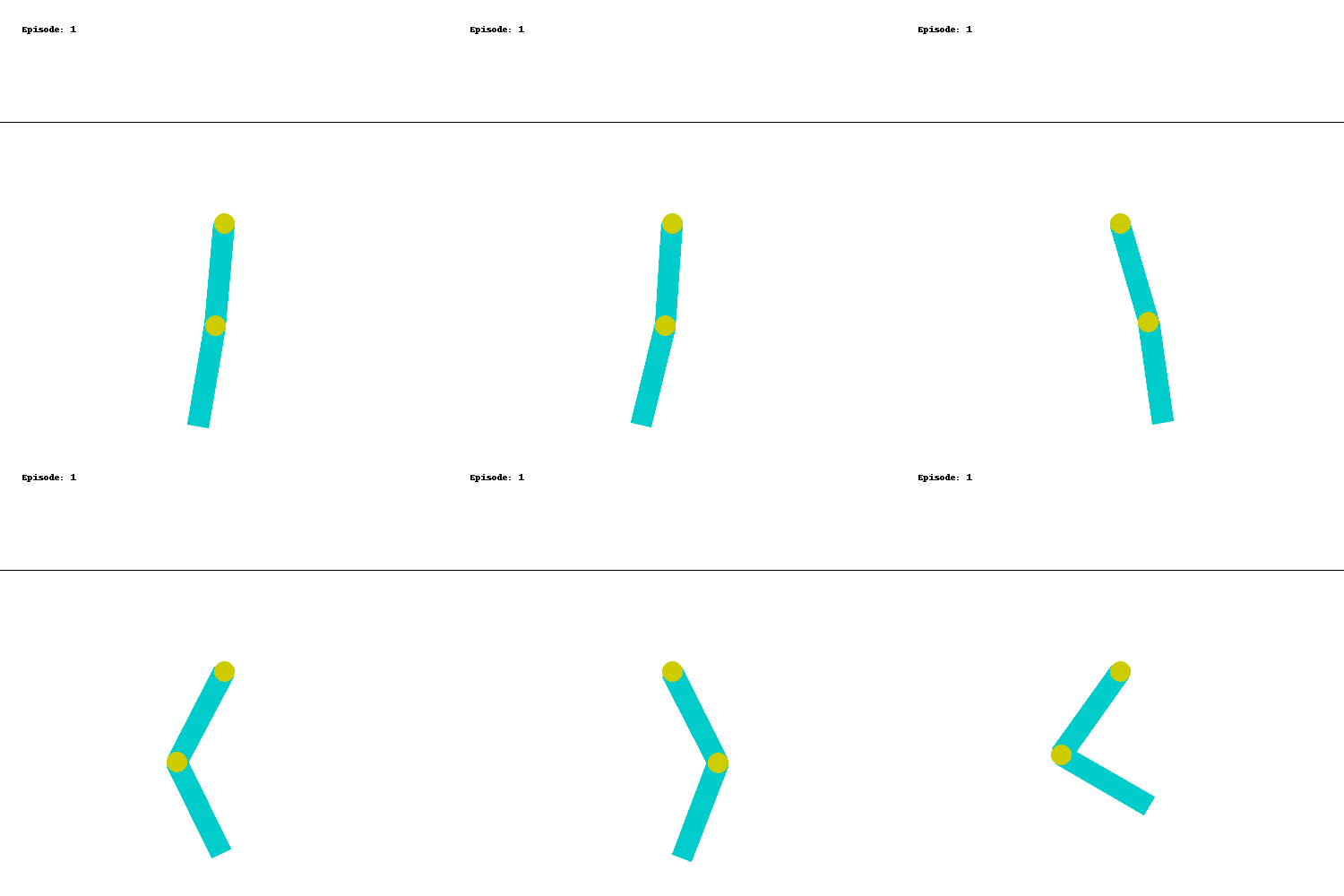
Each environment describes a game. The setup of the game of `Acrobot-v1` is as follows: There are two chain links hanging from a point, tied together, and each of the links can freely move within the reasonable bounds of the physical system. The objective is to apply force to the joint of these two links to ensure that the link touches a line above a certain height from the chain.

The observation space or the state for this game consists of some properties like linear and angular velocity of the chains and stuffs, (very complicated physics for me!), so we are just going to assume that it is simply a vector. There are only 3 possible actions at every time, push the joint to the left or to the right or do nothing.

While we take some random actions, you can see that the chain links just moves erratically and it does not achieve the objective. So, let us apply Q-learning and see whether we can make the agent learn to solve this game.

Before we do that, since the state is continuous, it is difficult to apply Q-learning right away, since we need to maintain a (state, action) pair table to store the Q-values. So, we discretize the entire state space into 10⁶ boxes, namely 10 grid boxes for each coordinate of the 6-dimensional state vector. The following Python function is doing that.

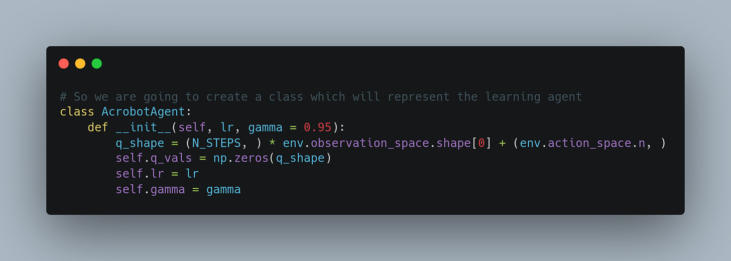
Now that we have a function to convert the continuous states to discretized state vectors, we shall write a class that represents the Acrobot playing RL agent. It shall have 2 functions, one for taking an action given the state and another for updating its Q-values.

The first function will be the function to get the action with the maximum Q-value. This is the Policy improvement step. The second function will be the one which updates the Q-values according to the Q-learning equation described above.

Now, we will try these Q-learning methods on the Acrobot game for 5000 episodes, with a learning rate of 0.01.

Once we perform these 2000 episodes, we try to save the agent's behaviour on a new episode and record that as a GIF image.

It looks like the agent is not learning anything. Wonder why is that? The behaviour still looks very random.

The reason is that only a very specific set of actions will lead to the correct goal. So, most of the time, the agent is not able to get any reward. Hence from the initial time itself, the Q-values are not updating much and staying at their initial values only.

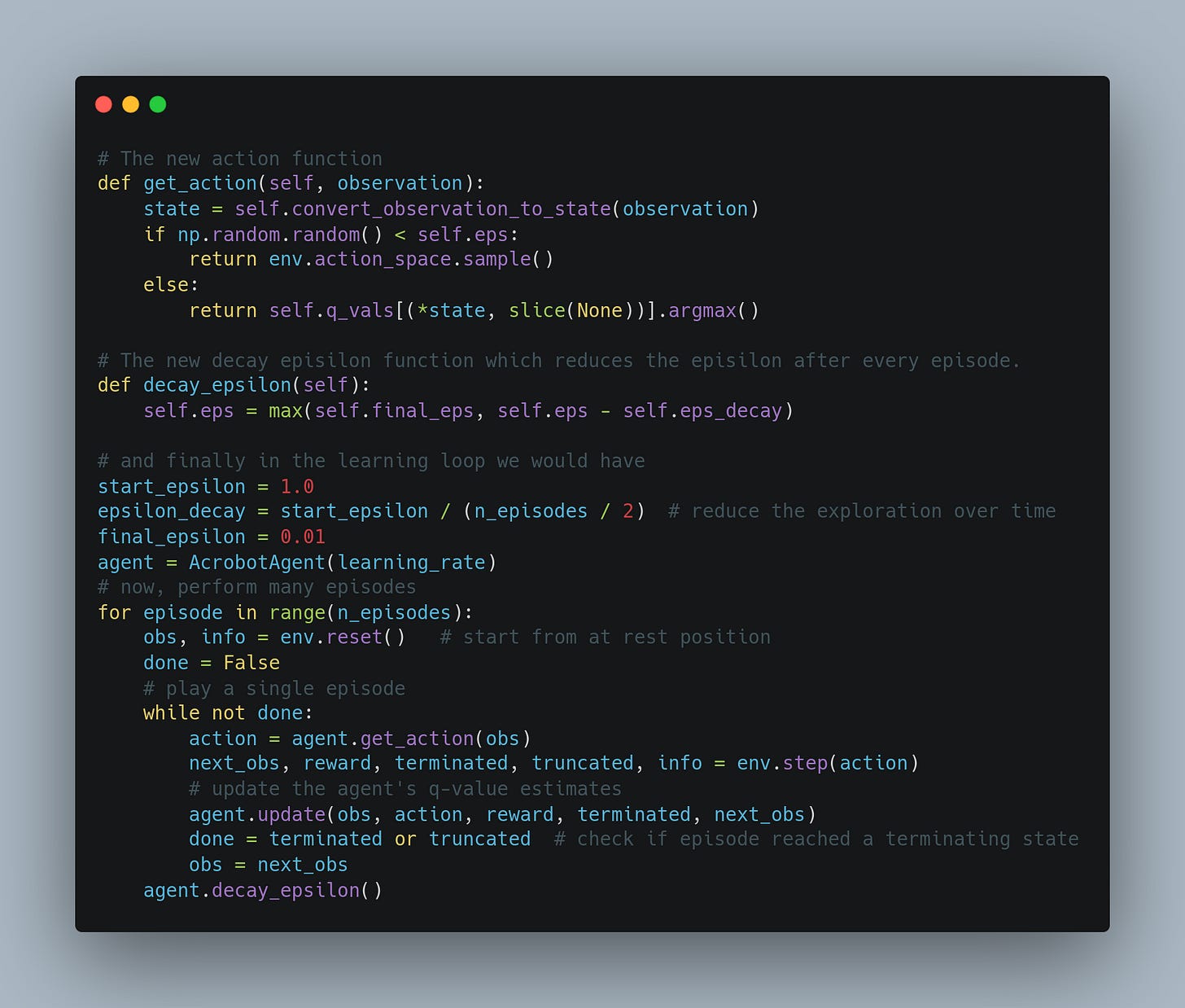
Instead, we can do the decaying 𝜖-greedy type strategy that we explored in the first post. Because in the initial episodes, we will be spending much time exploring the consequences of different actions, it is more likely to hit the target a few times and the rewards will propagate through the Q-values appropriately. As the episodes increase, we shall try to decrease the 𝜖 to reduce exploration.

So, here are the few modifications we need.

Now that we are exploring a bit at the beginning, we do 5000 episodes, and after that the result becomes very promising.

It is a bit hard to see that the chain link is touching the target line. Here's the final frame.

Q-Learning for Moon Landing?

Next, we will try the same method for the lunar landing environment present in the `gymnasium` package. It contains several continuous state-related information as before, and makes 4 actions: fire the left engine, fire the right engine, fire the main engine or do nothing.

Here's how the environment looks in action.

We tried the same thing as we did for the Acrobot game. We discretize the state space, and apply the Q-learning algorithm to train an RL agent. After 10000 episodes, this is the result.

Looks like it is failing pretty much. In between we have a few decent episodes though!

It seems that applying Q-Learning to the LunarLander environment presents some challenges compared to the Acrobot environment. Can you think of why? Please share your thoughts in the comments!

However, so far all the algorithms that we have explored uses a table to track down the Q-values for the state-action pairs. This is why we need to discretize the continuous observation into a state vector, which makes it lose a few pieces of information. In the next post, we shall learn different algorithms that we can use to solve reinforcement learning with these continuous state space and event continuous action spaces. Some of these algorithms include Proximal Policy Optimization (PPO), Trust Region Policy Optimization (TRPO) and Deep Q-Network (DQN).