

Encoding sentence meaning - Natural Language Processing Part 5
This post introduces the encoder-decoder type of architecture for all kinds of natural language processing tasks and discusses mechanisms of LSTM, GRU, etc.

Introduction
One of the fundamental studies in natural language processing is to understand the meaning of words, sentences and documents. We have seen one such way to do this for words, using embedding vectors, in the last post (in case you’ve missed it, here’s the link to the post). However, we also discussed the potential problems with simply aggregating the word embedding (tldr; a numerical vector representation of each word that describes its meaning) into an embedding vector for a sentence, as the ordering of the word, plays a very crucial role in defining the meaning of the sentence.
So the most common way to handle such dependencies for a natural language processing task is to have a “sequence-to-sequence” model, also popularly known as the “encoder-decoder” architecture.
Also, at this point, a basic familiarity with deep learning may be very helpful before we move on. Here’s a good introductory video by 3Blue1Brown.
Sequence-to-Sequence Model
The sequence-to-sequence model or encoder-decoder architecture was first introduced for the application of natural machine translation (NMT), the job of translating one language (e.g. - German) to another language (e.g. - English), which we currently use in our daily lives through Google Translate.
Such a system comprises two parts:
The encoder part: This part takes in the sequence of words (or the word embeddings), and combines them together to create a meaning representation of the entire sentence.
The decoder part: This part takes in the meaning of the sentence outputted from the encoder, and the previously translated text so far, to output the next predicted word (token). Think of this process like the keyboard suggestions one word at a time when typing something on your phone.
Since both of these part process sequences, together they look like you are taking a sequence of words and producing another sequence of words — so is the name sequence-to-sequence architecture.
Before diving deeper, let us understand a bit more about the applicability of these two components. Based on the NLP application you want to do, you will want to use one or both of these components.
Consider a sentiment classification problem. In this case, the meaning of the sentence should be enough to classify the sentence as “happy” sounding or “sad” sounding. So, you will need only the encoder component here.
Consider an application where the computer is given an image and it needs to come up with words to describe the image (things like this can help the visually challenged people). In this case, based on some process, you would already have a representation of the meaning of that image, and you only need to use the decoder to convert that meaning into words one at a time.
And, of course, applications like translation require both the encoder and decoder components.
Diving deep into Encoder
The encoder part encodes the meaning of the sentence into a numerical vector representation and also takes care of the word orderings. At a high level, it keeps a “memory” vector (to hold the meaning of the sentence), and keeps processing each word as it appears in the sentence to modify some or all parts of that “memory” vector. The final “memory” vector gives the numerical representation of the entire sentence (or the entire sequence of words).

Okay, now let us zoom in to understand what this “processing” really means. There are different ways for “processing”, and we will talk about each of them.
The Usual: Recurrent Neural Network
The usual recurrent neural network approach works like this. Let’s say, there are n words with embedding vectors, w₁,w₂,...,wₙ in sequence in the input. Also, let h₀ be the “initial memory” or “hidden state”. To compute the next hidden state, we simply take both of the current word vector and the previous hidden state, concatenate them, and then apply a linear combination (with parameters) on them with an activation function at the end, i.e., hₜ=𝜎(A × (hₜ₋₁|| wₜ)), where A is a weight matrix. Then, we keep fiddling with these parameters until we can use hₜ to predict the next word vector wₜ₊₁, for all index t of the sequence.
To understand at a high level, think about how we read a piece of text to understand its meaning. We read from left to right, one word at a time, and then keep conjuring up a meaning of what this piece of text is really about. And as you read more and more, you combine your existing understanding (existing hidden state hₜ₋₁) with the new word wₜ and then try to produce the new understanding (next hidden state hₜ).
However, you might say now what about Arabic or Urdu? Which we don’t read from left to right but from right-to-left?
For the same reason, you can consider a “bi-directional recurrent neural network” instead, as presented in this original paper by Schuster and Paliwal. In fact here’s a sentence:
She noticed the tear in his eye.
If you go from left to right, only after you reach the end word “eye”, you understand that the “tear” means crying, not ripping or cracking. In this case, a bi-directional RNN can pick up the cues from the end of the sentence and update the meaning. In a bi-directional RNN, the words in the sentence is processed from both left to right and right to left, and finally, the meanings (hidden states) are combined together by simple concatenation.
Here is a sample code showing the implementation:

Vanishing Gradients and Gated Networks
Around the end of twentieth century, researchers started to notice one major flaw with RNN - it starts with degrade its performance rapidly as the sentence length is increased. Behind that, the technical reason was something called “vanishing gradient problem”; let me explain what that is.
Let us consider the sequence of words: [How, old, are, you, ?]
Now, to perform the gradient descent algorithm in order to train this network, we need to calculate the derivative of the loss with respect to the parameters. The loss is measured only at the end of the sentence, when predicting the answer “I am … years old.” Therefore, by the chain rule of differentiation,
Which effectively tells that to measure the change in the loss (calculated only at the last word) for a unit change in parameter, you need to measure the change that a unit change in parameter makes to the meaning vector h₁ after processing the first word “How”, then multiply that change with the change it makes to the meaning h₂ (after processing the word “old”) for every unit change in h₁, and keep doing for every internal hidden state.
As an analogy, consider this example: for adding every worker in workforce, say the GDP of an imaginary country increases by 5 Bitcoins (suppose this is the traditional currency for the country). For every increase of bitcoin in the GDP, the tax revenue of its government increases by 0.2 bitcoin. For every unit increase in tax revenue, the government includes 10 people in the free healthcare program. Now, if you join the workforce, GDP increases by 5 BTC, which translates to (5 * 0.2) = 1 BTC increase in tax, which includes (1 * 10) = 10 people into the free healthcare program — effectively, the change you are making is measured by multiplying all these one-step changes.
Now usually, these one-step changes in RNN are very small, and hence, multiplying quite a few of them quickly makes it even smaller, close to zero. Which means, the gradient descent step does not update the parameters much, and your network learns nothing from the training data.
To counter this problem, in 1997, Hochreiter and Schidhuber came up with the idea of “Long Short Term Memory” (LSTM) and much later, in 2014, Cho et al. came up with the idea of “Gated Recurrent Units” (GRU). Both of these are based on a very basic idea: the separation of concerns. While the “hidden state” were used to hold the meaning vector of the sentence up to a particular point like a short term memory, an additional long-term memory (think of it as another vector) was included in the network to hold the meaning of the “terms” that may be relevant later on. For example, you might want the long-term memory to hold the “subject” to understand the form of verbs and pronouns that occur later in a sentence, or if it is a pronoun, it may occur even in the next few sentences.
Long Short Term Memory (LSTM)
The most prominent difference of LSTM over the existing architecture was the incorporation of a separate memory vector to hold long-term context, while the short term vectors hₜ were being processed as it is in RNN. Each such processing looks something like this:

Let us zoom in on the inner workings of this LSTM cell. The top line (with arrows) that goes from left to right is actually the long-term state vector, which gets passed from each cell to the next cell.
The leftmost part is where we first apply a sigmoid function on the input vector xₜ. Sigmoid is a special function that produces a number between 0 and 1, so you can think of it as a proportion of forgetfullness: 0 means it behaves like an alzheimer patient and forgets everything, 1 means it has a photographic memory and remembers everything. And, multiplying that number between 0 and 1 (e.g. a fraction like 0.3 say) with the long-term memory vector thus makes it like an average human - forgetful for some stuff (like the actual date of the anniversary), but retainer for eventful memories (like the experience on a date with your crush).
In the middle part, we have an operation mathematically described as: cₜ=cₜ + 𝜎(xₜ) × tanh(xₜ). The tanh(xₜ) creates values between +1 and (-1), indicative of the adjustments you should make in your memory. As an analogy, when you read an article or a new book, it usually enriches your memory and philosophies, but it does not overwrite them completely. The 𝜎(xₜ) now works in the opposite way of above, it picks value 1 on what adjustments are useful to commit to the long term memory, and finally, these adjustments are made by doing the addition with cₜ.
Now, for the third part, the LSTM authors consider an additional assumption, that the long term memory vector is expressive enough that it also contains the short term information. Thus, you see an arrow coming downwards from the long-term memory and getting filtered by the tanh(.) and 𝜎(.) functions, before outputting the next “hidden state” hₜ.
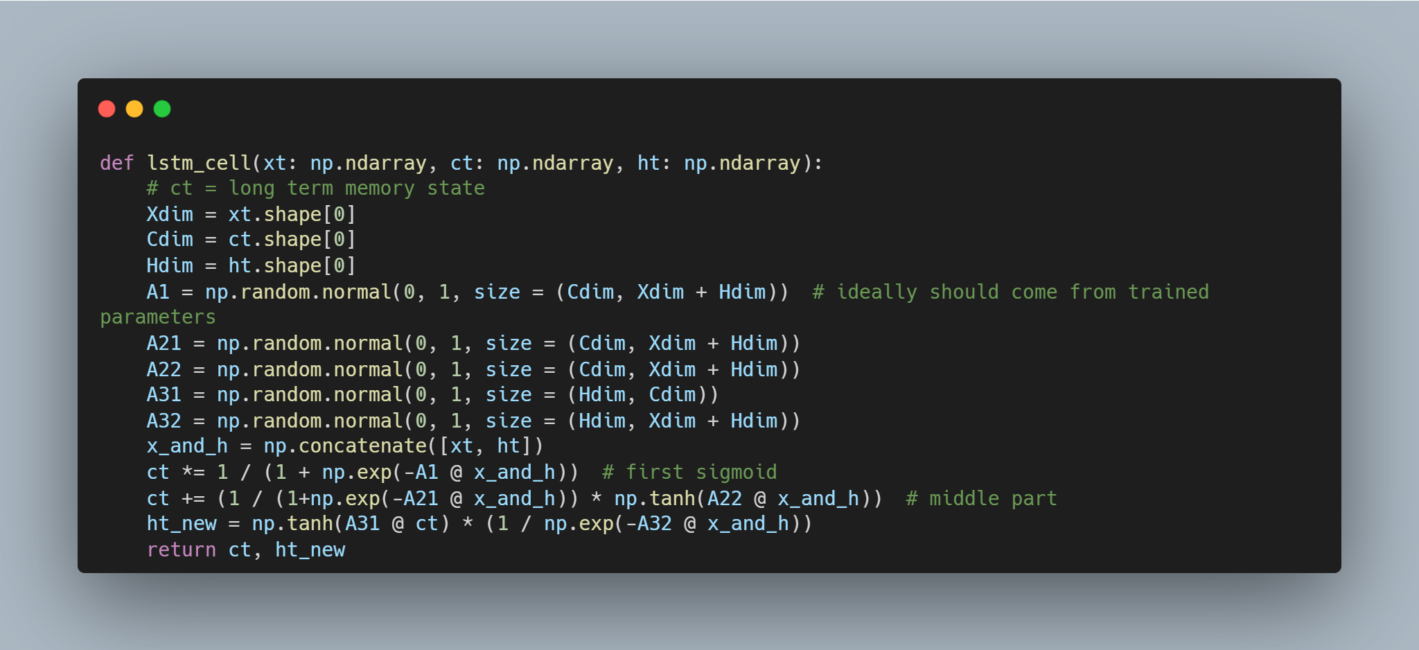
The following is a basic Python implementation of how an LSTM cell:
Gated Recurrent Unit (GRU)
While LSTM was able to capture long term dependencies in the sequence of words present in a sentence, it had a problem of memory requirements. This is because, instead of a single hidden state, now one needs to store the long term memory vector as well, which may present some bottlenecks if you are processing a large batch of sentences at once.
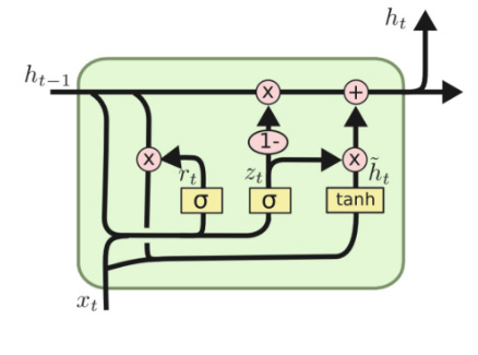
Instead of maintaining two hidden states (one for long term and one for short term), GRU aims to combine them into a single memory state. It is a bit “diverged” from how humans would understand, but it is needed to ensure that computationally, these neural networks are feasible to implement.
Let’s look at the middle part with the sigmoid. It is the same as the first part of LSTM, it updates the memory vector (shown at the top line) to forget some of the things. The usage of “1-” ensures the 𝜎(.) computes the things to forget (instead of things to retain).
Let’s now look at the first part and 3rd part together: hₜ += tanh(xₜ||𝜎(xₜ) × hₜ₋₁) × things to forget. The part 𝜎(xₜ) × hₜ₋₁ basically takes some of the coordinates from the memory vector, and makes the rest of them close to 0, and then a tanh(.) computes the adjustments to make in the memory as before. However, since GRU uses the same vector to hold both long term and short term memory, it only needs to update the coordinates where it has forget something from step #1. Hence, we multiply that by the sigmoid (note that it is not the (1 - sigmoid), but rather the sigmoid itself) and add these adjustments finally to the memory vector.
A basic Python implementation of the GRU cell will be like this:

Conclusion
Recurrent neural networks (RNNs), along with their advanced variants like LSTMs and GRUs, have played a crucial role in modelling sequential data by capturing contextual dependencies. Their designs mimic how we humans process the natural language — one word at a time, refining our understanding as we go.
However, this sequential structure has been a bottleneck for RNNs. Each step of the RNN depends on the previous step, therefore, even with the advent of good hardwares like GPU, which can parallelise billions of computations per second, it is still slow compared to our expectations. Think about that how it takes us days / weeks to read and understand a book, while Chatgpt can understand and summarise in seconds.
This led researchers to look for more efficient architectures — ones that could process all words simultaneously, and find out key words to pay “attention” to. And that led to the development of attention mechanism, and later transformers architecture, providing a game-changing idea that built ChatGPT. In the next post, we will explore this in detail, and understand the intuitions behind it.
And as always, thanks for being a valued reader! 🙏🏽
Until next time.