Latent Dirichlet Allocation on the New Year’s Resolutions - Natural Language Processing Part 3

My last post on the NLP series (see here if you have not already) covered a pretty basic way to identify the topics present in various X posts about New Year’s resolutions. However, we also identified the shortcomings of this basic exercise using Latent Semantic Analysis (LSA), namely:

• The resulting word distribution in each topic was very noisy.

• Multiple topics were allowed to share many of the words, there was no clustering and much less of a clear pattern.

One of the reasons for this was that we understood the topics and the words as “linear” combinations of each other, while the connection between them is actually a bit more nuanced and probabilistic in nature. In this regard, David Blei, Andrew Ng and Michael Jordan came up with this seminal work on Latent Dirichlet Allocation.

The Basics

Before we dive deeper into this, let us first get familiar with some notations and relevant concepts.

• The vocabulary contains V different words. Each word w is represented by its one-hot encoding vector with respect to this vocabulary.

• A document (or X post) is simply an ordered sequence of these words, one after another. A document d with n words are denoted as (w₁,w₂,...,wₙ).

• We have a collection of M different documents (or X posts).

• There are K latent topics, think of each topic as a probability distribution over the vocabulary.

To understand the last part a bit more, consider the simple example where our vocabulary consists of 5 words, {sea, river, bank, money, cash}. I can think of at least 2 different concepts underlying these words, one about “natural things related to water” and another about “financial stuffs”. Specifically note that, the word “bank” can have two different meanings, relating to both these topics. As a result, you can think of these topics as the following probability distributions:

• “Natural Things”: P(sea) = P(river) = P(bank) = 1/3, P(money) = P(cash) = 0.

• “Financial Things”: P(sea) = P(river) = 0, P(bank) = P(money) = P(cash) = 1/3.

With this notion of viewing the topics as a probability distribution, think about the process of how an X user called Mr. Bond, who is writing the post is coming up with the post.

1. Mr. Bond first thinks about what “topics” he wants to write about. Mathematically, you can think of this as choosing a probability distribution over the list of topics.

2. Then Mr. Bond thinks about how long the post he wants it to be. This means, mathematically we choose the size of the post “n” according to a discrete probability distribution.

3. Now for each word that Mr. Bond wants to write.

   1. A topic is first chosen, according to the probability distribution selected at step #1.

   2. Then based on the topic, he chooses one word according to the probability distribution of that topic. (To give an example, let’s say I choose to talk about “financial things”, then I choose a random word between “bank”, “money” or “cash”.)

Notice that, we must get rid of stopwords and prepositions and conjunctions which usually do not belong to any topic, but rather are required to ensure proper grammar of the sentence.

Now, in the LDA paper, the authors consider specific types of probability distributions in steps #1, #2, and #3. Namely:

1. Probability distribution over the topics: 𝜃 ∼ Dirichlet(𝛼)

2. Probability distribution over the size of document: n ∼ Poisson(𝜉)

3. Probability distribution for choosing a topic: zₖ ∼ Multinomial(𝜃)

4. Probability distribution for choosing a word: wᵢ ∼ p(w∣ zₖ, 𝛽), the specific topic distribution.

In statistical terminologies, such description of the data generation process is called “Hierarchical models” and the typical way to solve and get the estimates of the unknown parameters (namely 𝛼, 𝜉, 𝛽) is using the Bayes theorem and a special technique called Gibbs sampling.

Here’s a very nice pictorial description of the dependencies between these parameters, from the original paper.

Some Intuition about the choice of priors

The specific choices of the different probabilities above determines some kind of “prior” knowledge about the data generation process, before even you see the data. It is useful to know how it affects our final analysis, and get a bit more intuition of what’s going on with these choices.

Dirichlet Prior

We consider each document to be a mixture of topics (turns of this mixture of stuffs is a very powerful technique, even in the recent LLM advancement with DeepSeek where they use a Mixture of Experts model), and this mixture is modelled by a Dirichlet distribution, which takes a parameter 𝛼.

A good analogy to understand this parameter 𝛼 is to consider the following: Suppose you want to paint your house, and for that you are mixing three colours (Red, Green and Blue) in a random proportion.

• If you stir them gently, you get a dominant colour (like a document focusing mostly on one topic).

• If you stir vigorously, you get a balanced mixture of all colours (like a document that covers many topics evenly).

• The Dirichlet parameter 𝛼 controls this mixing behaviour.

Coming back to our specific example of documents generated from a mixture of topics, we have something like:

• Small 𝛼 (< 1.0) → Documents tend to focus on one topic, e.g. Legal documents maybe 100% about the law.

• Medium 𝛼 (~ 1.0) → Documents with a mix of a few topics, e.g. Like this blog post, a bit of math and a bit of computer science.

• Large 𝛼 (> 1.0) → Documents that cover many topics, e.g. a news article that talks about politics, economy, sports, celebrity gossips, etc.

Here is a graphical visualization of this, for the probability distribution over 3 topics with different choices of 𝛼.

Poisson Prior

The choice of Poisson prior is more natural when modelling the length of the document (or X post). Many empirical studies have shown that the document lengths usually have an exponentially decaying probability distribution, which for count data transforms into a Poisson distribution. To convince you further, let us see the histogram of the length of X posts of the new years resolution data.

The exponentially decaying tail now should convince you why n ∼ Poisson(𝜉) is a “good” choice of prior.

The Inference

Once we have the above data generation process, we would like to obtain the estimates (or posterior distribution, i.e., the probability distribution over the likely values of the parameter that could have generated the data that you are seeing right now!) of 𝛼,𝛽,𝜃.

If you are familiar with a bit of conditional probabilities, here’s what you want:

\(p(\theta, z \mid w, \alpha,\beta) = \frac{p(\theta, z, w \mid \alpha, \beta)}{p(w \mid \alpha,\beta)}\)

Here, we only show the probability distribution of unknown 𝜃, given the other two parameters. While the numerator can be easily computed as:

\(p(\theta, z, w\mid \alpha,\beta)= p(\theta \mid \alpha)p(z \mid \theta)p(w \mid z, \beta)\)

and all of these components can come directly from the data generation process. However, it is not so easy to evaluate the denominator, and this creates a lot of problem.

One solution that is proposed in the paper is to use a technique called “Variational Inference”. What it tries to do is to produce a sequence of tractable probability distributions that becomes closer and closer to the target probability distribution over a sequence of iterations. For instance, here we want to find the posterior distribution p(𝜃,z∣w,𝛼,𝛽) (i.e., the distribution of the topics given the words in the documents), but we will appropriate it with another distribution q(𝜃,z∣𝛾,𝜙) which is actually “free of the data”, at least initially. Now what we try to do is to modify the parameters 𝛾 and 𝜙 so that the probability distributions p(𝜃,z∣w,𝛼,𝛽) and q(𝜃,z∣𝛾,𝜙) match — and one way to do that would be to minimize the Kullback-Leibler divergence between them — which, in turn, starts producing a dependency with the “observed words” through this minimization.

If you are mathematically inclined, you might want to do a bit of calculation to figure this out yourself, but here’s what the algorithm turns out to be:

1. Initialize a random assignment of each word to one of the k topics.

2. For each word in the corpus, update its topic assignment probabilities based on:

\(P(z_i =k \mid z_{-i}, w) \propto \frac{n_{k,d} + \alpha }{n_d + K\alpha} \frac{n_{k,w} + \beta}{n_k + V\beta}\)

where K = # of topics, V = # of words (vocabulary size), n denotes the number of times the word “w” satisfies a requirement (and that requirement is given by the suffixes, i.e., suffix “d” is # of times the word appears in the document “d”, and suffix “k” is the # of times the word “w” is assigned to a topic “k”). — I am leaving out a lot of details here, just for the sake of simplicity!

3. Sample a new topic for the word based on this probability distribution.

4. And keep repeating until convergence.

I think it was a lot of theory till now, but let’s get some action by running this LDA process on our dataset. Note that, we could perform these iterations using a normal for loop in Python, but fortunately, the Sklearn library provides a very optimized implementation of this algorithm.

LDA for New Year’s Resolution Data

To begin with, we do the same preprocessing and cleaning step as before, so I am skipping that part. Once you have the cleaned X posts, you can pass that as a list to the fit method of an instance of LatentDirichletAllocation class as shown:

Here, we choose to consider K = 10 topics. Next, to find out what these topics are comprised of, we can look at the lda_model components (i.e., the probability distribution for each topic), and consider the top few words for each topic. Here is the list that comes up.

Topic 1: fo, meet, live, life, amp, time, need, family, let, things
Topic 2: new, resolution, years, going, change, people, bette, resolve, use, yea
Topic 3: eat, weight, lose, new, healthie, like, yea, food, resolution, look
Topic 4: want, yea, love, fo, newyea, tweet, awesome, time, new, living
Topic 5: stop, smoking, right, rt, cigarettes, quit, think, club, suppe, buy
Topic 6: start, new, resolution, gym, yea, day, rt, years, social, week
Topic 7: finally, finish, eve, job, happy, fo, gonna, book, cut, enjoy
Topic 8: make, possible, money, thanks, say, learn, friends, god, good, fo
Topic 9: drink, wea, game, fit, rt, fat, read, coffee, ready, yea
Topic 10: years, resolution, new, rt, yea, resolutions, fo, make, spend, like

Well, the topic distribution looks more reasonable that what we achieved before using Latent Semantic Analysis in our previous post, but there are still some problems. And one of the crucial problem that I can find is the following: Some words (e.g. “fo”, “yea”) appear multiple times in different topics.

So here’s how I would approach this (think again with a Bayesian mindset that we needed to perform LDA).

• We are considering here P(word | topic), and for each probability distribution, we are looking at the words for which these probabilities are high.

• However, for a word like “yea”, may be P(word = “yea” | topic 4) = 0.4 and P(word = “yea” | topic 6) = 0.25. If that’s the case, then when we observe the word “yea” in a post, it is much more likely that it would have probably come from topic 4 instead of topic 6. (I know some mathematicians will scream at me at this point for saying this, but please bear with me for a sec!)

  • However, to actually precisely say this, you need to consider the reverse conditional distribution, i.e., P(topic | word = “yea”).

  • This is where we can use Bayes theorem.

• Finally, for each word we would assign it to a particular topic based on this probability distribution P(topic | word).

• Once we have this assignments, we can think that the corresponding word is removed automatically from all other topics, hence we would end up without any overlap.

And here’s how we can do this in Python.

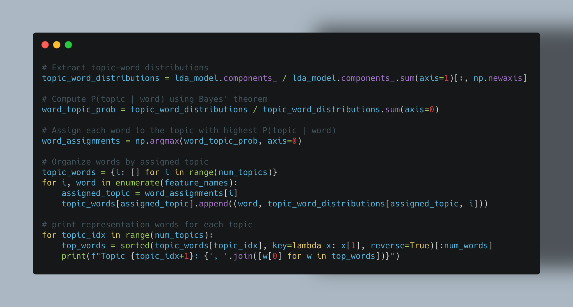
And the result is:

Topic 1: fo, meet, live, life, amp, time, need, family, let, things
Topic 2: going, change, people, bette, resolve, use, person, try, nice, twitte
Topic 3: eat, weight, lose, healthie, like, food, look, books, play, hashtagoftheweek
Topic 4: want, yea, love, newyea, tweet, awesome, living, follow, health, instead
Topic 5: stop, smoking, right, cigarettes, quit, think, club, suppe, buy, drinking
Topic 6: start, gym, day, social, week, watch, lbs, days, actually, tomorrow
Topic 7: finally, finish, eve, job, happy, gonna, book, cut, enjoy, wanna
Topic 8: make, possible, money, thanks, say, learn, friends, god, good, close
Topic 9: drink, wea, game, fit, fat, read, coffee, ready, stay, month
Topic 10: years, resolution, new, rt, resolutions, spend, perfect, girl, everyday, break

I believe this is much more clearer than the previous one. For example, I see:

• Topic 1: Live life and make time for family.

• Topic 2: Trying to be a nice and better person.

• Topic 3: Eat healthy food, lose weight.

• Topic 5: Stop smoking cigarettes, and clubbing.

• Topic 8: Make friends, be thankful, learn more and make money.

And so on.

Possibly you still see some overlaps, so may be you are thinking that 10 topics are too much. We can probably reduce it. I though so to, so here’s what I did additionally, I considered the probability vector (from the probability distribution over the vocabulary) for each topic, and then calculate cosine similarity between them (technically, may be a Kullback Leibler type divergence measures would have been more appropriate). Turns out, the similarity between different topics are not that great, so may be (just may be), K = 10 is a possibly right choice.

Conclusion

In this post, we learnt about a new technique for topic modelling, called Latent Dirichlet Allocation (LDA). We analyzed the New Year’s resolution dataset with it. But let’s take a time to think about the pros and cons.

• LDA does not take care of synonyms. For example, two words “Hi” and “Hello”, although synonymous, are treated as separate words by LDA due to the one-hot encoding representation of the words.

• How do we determine the number of topics?

• Is there is measure to understand how good we have performed for this task of finding out the topics? How do I know if I have detected the correct topics or not? (In contrast, for learning to classify cats and dogs, I can measure accuracy as a measure of performance.)

In the next few posts, we will explore the answers to these questions. Till then, stay tuned for more.

---

Thank you very much for being a valued reader! 🙏🏽

Like, share and subscribe to get notified when the next post of this series is out!

Until next time.