The topics of New Year resolutions - Natural Language Processing Part 2

In the last post (see here if you haven’t already), we discussed a basic premise of Natural Language Processing, and how we can use it to analyse posts (formerly known as tweets) on X to find out the trends and keywords in New Year resolutions.

However, our analysis faced several challenges. One of them was that different words like “joy”, “happy”, “bliss”, refer to the same idea or concept. Now suppose, we find the counts of these words in 20s, but the most occurring word “new” appears 50 times, then we would see a distorted view if we consider the most frequent words (or the words with the most tf-idf). Thus, in this post, we will go one step further, and try to understand the concepts (or topics) behind these posts, and not just look at the counts of each words.

Document Term Matrix

As you probably know, most of statistical data analysis starts with a dataset, usually in the form of tabular (or rectangular) data with multiple rows and columns. But in the case of NLP, here we are simply given a list of texts. Naturally, our first step of the analysis should be to convert these texts into some form of tabular data that we can analyse. And the representation that’s going to help us is called the “Document Term Matrix” (or DTM for short).

Each row of the DTM corresponds to a document (in this case, a post).

Each column of the DTM corresponds to a term (i.e., word in the vocabulary).

Then, the first version of DTM, as conceptualised by Harold Borko, corresponds to a sparse matrix where we put a nonzero value “x” at the intersection of row for document “d” and column for word “w” if the word “w” appears “x” times in the document (or post) “d”. Everywhere else, we put a value of 0.

This is an example from the same paper where the author shows part of DTM for a set of documents containing abstracts of some journal articles related to psychology. (A significant portion of the initial development of NLP was carried out by psychologists who were also good with numbers!)

Note that, each of the nonzero numbers is actually the term frequency of the column-indexed word in the row-indexed document.

As we saw earlier in the last post, A much better measure is to consider tf-idf which normalizes the term frequencies by the inverse document frequencies to penalize the words that are present almost everywhere. This gives rise to a modified version of the DTM considered above, which is also the standard version currently used for most purposes. In mathematical terms, this means the entries of the DTM are:

\(\begin{align*} M_{d,w} & = \text{tf}_d(w) \times \text{idf}(w), \text{ where }\\ \text{tf}_d(w) & = \dfrac{\text{# of times word } w \text{ appears in document } d}{\text{# of times word } w \text{ appears in entire corpus}}\\ \text{idf}(w) & = \log\left( \dfrac{1}{\text{# of documents containing word } w} \right) \end{align*}\)

Since I already demonstrated how to calculate the tf-idf scores in my last post, I am going to use a more high-level utility function from the Sklearn package to do this. And here’s a Python code snippet to calculate the DTM.

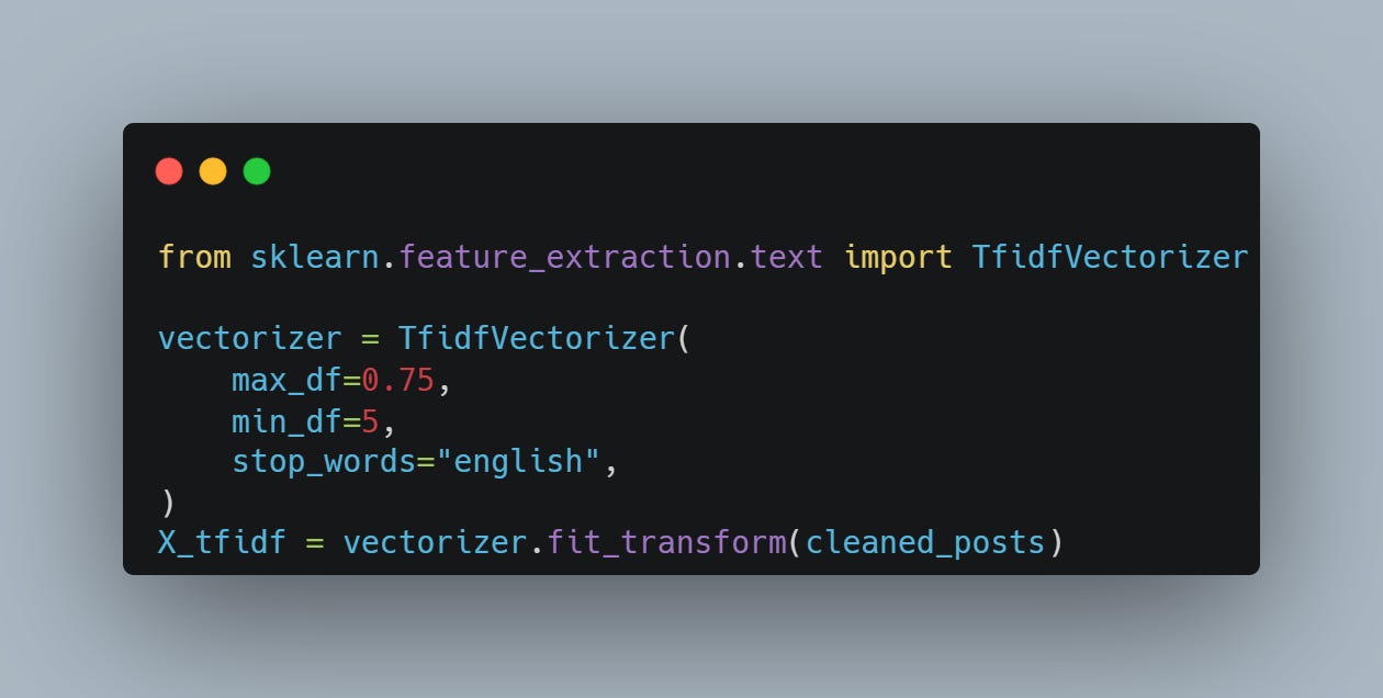
Here, we use the min_df = 5 and max_df = 0.75 to ignore all words that appear either in less than 5 posts or more than 75% of the posts. It turns out, only 0.5% of the resulting X_tfidf matrix (5003 rows and 933 columns) has nonzero entries.

How to use this DTM?

Now, we are going to dive deeper into more mathy stuffs. Let’s recap once more: so far, we have a document-term matrix, where we have documents in the rows, words in the columns, and each entry corresponds to the tf-idf of the corresponding word in that document.

As our goal is to understand the topics of the documents, let’s try to define the topics in a more mathematically concrete way. You can think of a topic as a collection of words: For example,

• When you mention the topic “sports”, you are thinking of some keywords like “cricket”, “football”, “chess”, “swimming”, etc.

• When you mention “bollywood”, you are thinking of “Amitabh Bachchan“, “Shah Rukh Khan”, “Hritik Roshan”, “Akshay Kumar”, “Katrina Kaif”, “Deepika Padukone”, and many others.

And so on. You get the gist.

However, one thing to note here is that, when I mention “sports”, if you are as prejudiced as me, then you are probably thinking less of "chess" and more of "cricket" or "football". Similarly, when I mention “bollywood”, you are less thinking of Anurag Kashyap, or Amit Roy (cinematographer) than the names I mentioned above. Therefore, every topic is not just a collection of words, but rather it’s a weighted collection. And instead of collection, we shall replace it with a weighted linear combination (as that’s the straightforward way to mathematically combine stuffs).

Therefore, you can think of a topic as

\(\text{topic}_1 = w_1 \times \text{word}_1 + w_2 \times \text{word}_2 + \dots + w_n \times \text{word}_n\)

And when a particular word should not belong to a topic, we can set the corresponding weight equal to 0.

At this point, we will use a bit of matrix algebra lessons. If you write the above equations for each and every topic, you should be able to invert these equations to solve for each and every word (if you want to be nerdy, assume some non-singularity conditions so that the matrix is invertible). Then you would essentially get

\(\text{word}_1 = u_1 \times \text{topic}_1 + u_2 \times \text{topic}_2 + \dots + u_k \times \text{topic}_k\)

This means you can think of each word as a linear combination of various topics. For example, when I mention the word “ball”, you are thinking of “sports” (e.g. football), a bit of “dance” (e.g. ballroom), and a bit of mathematics (e.g. ball of epsilon-neighbourhood), and possibly many related topics. Therefore, each word is also a weighted linear combination of various topics.

On the other hand, a document is a piece of text, which may mention multiple topics. For example, a newspaper article about “Celebrity Cricket League” will mention both the topics of “sports” and “celebrities” (or “bollywood”). Therefore, by a similar logic as before, we may be able to write each document as

\(\text{document}_1 = v_1 \times \text{topic}_1 + v_2 \times \text{topic}_2 + \dots + v_k \times \text{topic}_k\)

Therefore, essentially the problem boils down to:

• Find a list of topic vectors.

• A linear combination of these topic vectors should give us the row vectors corresponding to the documents.

• A linear combination of these topic vectors should give us the column vectors corresponding to each word.

In mathematical terms, we call this a “Factor model”. And when you solve it, all NLP analysts will call this as the Latent Semantic Analysis (LSA). Here’s a very good animated video of this LSA process happening and some additional clustering so that it is easier to see the topics to convince you of this process.

With a bit more imaginative power and some training in mathematics, you will be able to see that this problem is the same as finding out an approximate rank factorization of the document-term matrix (or more precisely, a singular value decomposition), which factorizes the DTM matrix M as

\(M = UDV^t\)

where U and V are orthogonal matrices and D is a diagonal matrix with its diagonal entries arranged in descending order. You can use the good ol’ numpy library to perform this SVD step.

U, D, Vt = np.linalg.svd(X_tfidf.toarray()) cumulative_variance = np.cumsum(D**2)/np.sum(D**2) plt.bar(x=np.arange(1, len(D) + 1), height=cumulative_variance, width=0.5) plt.show()

And this yields what’s known as the “scree plot”, which shows the contribution of variance explained by the most prominent combination of words.

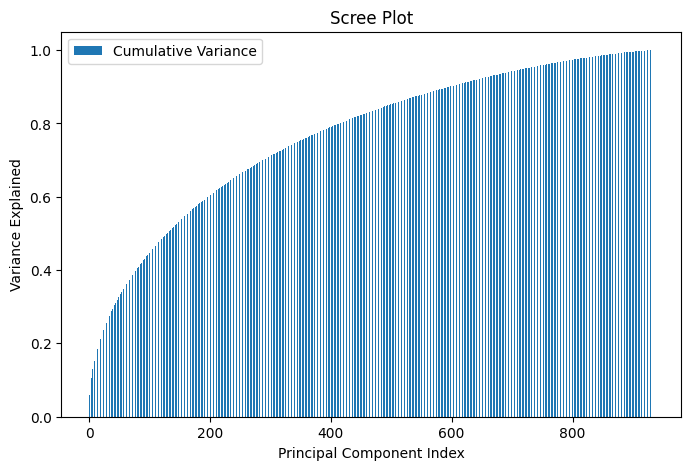
This shows a clear picture now that using only the first 200 top linear combinations of words, you can explain about 60% of the variance of the different combinations of topics present in the posts. And now, the big reveal: To understand what words make up most of each topic, we are going to look at the matrix DVᵗ to find out the weighted linear combinations of the words. And then, we are going to look at those words for which the coefficients are either largely positive or largely negative.

In mathematical terms, if we have that the topic “k” is generated as

\(\text{topic}_k = w_1 \times \text{word}_1 + w_2 \times \text{word}_2 + \dots + w_n \times \text{word}_n\)

We would pick up the few words for which the magnitude of wᵢ is larger. Here is a Python utility function that does exactly this.

At this point, if I print the first few topics, we get:

Topic 1: new resolution years yea stop make like eat happy people Topic 2: make yea money possible thanks years time stop resolution going Topic 3: stop yea smoking cigarettes suppe club right new people eating Topic 4: time yea like amp people start life stop bette spend Topic 5: like bette eat time amp want love yea life start

Although the topics overlap, we get two major ideas: One is that people want to make money, eat properly and be happy in general, and spend money for their loved ones. Another is to stop smoking cigarettes and go to clubs to meet new people instead. This was the resolution topic from 2015.

And once we did the same analysis with the posts from 2021, we get

Topic 1: year love thank wish good hope best great wishing years Topic 2: happynewyea best newyea family friends wishing good hope happiness health Topic 3: hope thank happynewyea good best great bette newyea love family Topic 4: thank hope good happynewyea great bette let morning god years Topic 5: family best friends wish wishes hope good wishing happynewyea amp

Clearly, it shows a different picture due to the presence of Covid19 pandemic. People are just wishing New years, spreading hope and love, and praying to God to make everyone stay healthy and get better.

Conclusion

In this post, we learnt about the first step in NLP, i.e., to create document-term matrix. We also learnt a technique called “Latent semantic analysis” (LSA) which allowed us to obtain a structure of the underlying topics. However, as we much, there are many overlaps between these topics and the result was not completely noise-free. One of the major problem was that the weights of the linear combinations that derive the topics from the words are not constrained in any way. So, multiple topics were allowed to share many words which are similar to each other.

Therefore, in the next post, we will look at some alternatives to LSA which will allow us to apply some clustering to ensure better segmentation of the topics. Maybe, some more interesting insights will emerge!

---

Thank you very much for being a valued reader! 🙏🏽

Subscribe and follow to get notified when the next post of this series is out!

Until next time.