

Text generation from machine understanding - Natural Language Processing Part 7

Introduction
In the last few posts of the NLP series, we understood how a text-to-text system (like ChatGPT) understands the meaning of the input sentences through a combination of embedding mechanisms and encoder type neural network. Now, we look at the other side of the coin, namely the decoder type architecture, which takes such a representation and comes up with the actual sequence of words as the output.
Decoding
The term “decoding” simply means to convert the internal vector-based representation of a system’s final thoughts back into the human-readable language. This is a key integral part of the entire NLP seq-to-seq system. Because here, in the first part, when the human-language words and sentences are converted into embedding vector representation for processing, nobody other than the system possibly understands what these vectors mean. Hence, unless it can be decoded back into human-readable form, the entire system for communication remains broken.
As an example, think of how you talk to your pet dog. When you say it to “sit down” in english, it understands it by converting it into some mental representation that only it understands — and you know it because your pet now obeys the instruction and sits down — but if it barks back at you, you don’t have a clear way to understanding what it means as it is not in a language that you understand. The first part is “encoder” — it is useful for you to instruct, but the second part “decoder” — is essential for communication.
The mathematical model of decoding
Just like us, current systems primarily output one word at a time. Suppose that you ask a question to an LLM system, say “How are you?”. Then, the LLM internally processes it as follows:
Input: “How are you?” => Output: “I”
Input: “How are you? I” => Output: “am”
Input: “How are you? I am” => Output: “doing”
Input: “How are you? I am doing” => Output: “fine”.
Input": “How are you? I am doing fine” => Output: <EOS>
Here, <EOS> is the special end-of-sentence token that is returned when the LLM thinks that it is done with the generation of the answer. However, what it really shows is the nature of how all the outputs of an LLM are generated as one word at a time, and each time the generated word is further fed back as part of the input into the LLM. This technique is called “Autoregressive decoding” in the current literature of large language modelling.
Mathematically, say we have already generated the words, w₁, w₂, ..., wₜ₋₁, then
However, I did make it a bit simpler before. Instead of just outputting the word directly, the system processes all the words before it and produces a probability distribution over the vocabulary, shown here as Pₜ. And then, the next word wₜ is generated by some strategies from Pₜ.
The reason is like this: Consider the partial sentence, “The weather is”. The next word could either be “sunny” or “rainy”, and if no context is present, then both are equally likely. But in the presence of some context, say, “I have never seen so much pouring, the weather is”, the next word is very likely to be “rainy” instead of “sunny”. Therefore, it is not always the case that there is one correct word to put in; there are always multiple choices, and some are “excellent” or likely, some are “good”, and some are “unlikely”. This is represented by using the probability distribution Pₜ.
From probability distribution to words
Greedy Decoding
The most common approach to decoding word wₜ from the probability distribution Pₜ is to take the most likely word. This means, for the partial sentence “The weather is”, among the words “sunny” with probability 55% and “rainy” with probability 43% and other words sharing 2% probability, we will always use the same word “sunny” as it has the largest probability. That means, the system, when asked, will always tell the same joke! 😏
Here’s a nice visualisation from this huggingface blog about greedy decoding.

There’s another bigger problem, though. This “greedy” method is very prone to getting stuck in loops. For example, consider the sentence, “I am happy because”; the next two words are probably another “I am” (e.g. I am happy because I am going on a trip today). So now, once you complete, “I am happy because I am”, the next likely word could again be “happy” (as the recent words “I am” usually follow with “happy”). So you end up with the loop:
I am happy because I am happy because I am happy …
Top-* sampling
At this point, you may ask, okay what if instead of always picking the word with the highest probability, what if I consider the top 2 choice of words and pick one randomly from it. In this case, the partial sentence “The weather is” can be completed with both “sunny” and “rainy”. This is the key idea of Top-K sampling, presented in this paper from Facebook AI Research group in 2018. They considered K = 10, i.e., at each point, they picked up the words with the 10 highest probabilities, and then further randomly select from these words by sampling from this restricted set of words.
Another similar idea came up in a paper by Holtzman et al. in 2020, which introduced the idea of top-P sampling (also called the nucleus sampling). One problem with the top-K sampling was the choice of K, which is very sensitive in the ultimate generation of the text. Rather, a more common sense approach is to take words that make up most of the probability distribution, say the 95% of it. For example, consider the two cases:
Input: The weather is. The output probability distribution is: P(sunny) = 0.55, P(rainy) = 0.42, P(cloudy) = 0.02, …. Here, taking the top 2 words “sunny” and “rainy” itself covers (0.55 + 0.42) = 0.97, i.e., more than 95% of the probability. Hence, sampling happens from these two words, “sunny” and “rainy”.
Input: I am. The output probability distribution is: P(happy) = 0.4, P(sad) = 0.25, P(depressed) = 0.15, P(fine) = 0.15, P(eating) = 0.03, …. Here, we need to take the top 4 words (happy, sad, depressed, fine) instead to reach 95%. Note that, this is now equivalent to K = 4 sampling.
This shows, top-p sampling dynamically adjusts the K in top-K sampling, based on a simple notion of ensuring the bulk of the probability distribution (i.e., the most possible words) are considered.
Beam Search
Beam search is another very popular decoding algorithm, introduced first in the paper by Lewandowski, Bengio (one of the bigshots of deep learning, you’ll find him almost in every big) and Vincent in 2013. This was initially developed to create new musical sequences; you can think of each “sargam” (or basic notes) as one of the possible “token” that can be used. What they understood is that instead of generating one word at a time and taking it according to a greedy algorithm, a more clever approach would be to look-ahead a few more words in future, and based on that decide what word to use for the current position.
Let me give you an example: Consider a partial sentence, “I am trying”. Some very likely next words are “it” or “this” — I am trying this. However, if we pick a less likely word “to”, we can add another likely word “create”, which will make the partial sentence “I am trying to create…”, which sounds more meaningful and likely to be used.
Beam search considers this idea. It considers n possibilities for each word, and after a length of m words, it calculates the likelihood of the entire sequence, using the conditional probability formula
And picks the m-length sequence of words that maximises this likelihood. In the above example, P(this, <EOS> | I am trying) < P(to, create | I am trying), so the phrase “I am trying to create” will be selected.
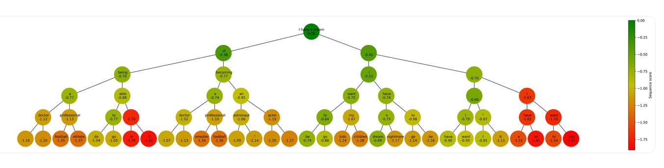
Here’s a nice visualisation of beam search from the same blog post. Compare this with the figure for greedy search: Essentially, beam search considers multiple options at each point, and hence it results in a search over a tree-like structure for the most likely sequence of words.
Contrastive Decoding
In September 2022, another group of researchers came up with another novel proposal for a decoding strategy. They mentioned in their paper that the top-K sampling or the nucleus sampling suffers from one key bottleneck. As it tries to sample the not-so-likely tokens as well, as the sequence of the generated tokens gets longer and longer, the sampled text may become diverse from the original text or even contradict itself. Clearly, the greedy algorithm avoids this problem, except that it creates the repetition problem instead.
Therefore, the key idea of their algorithm is to try to select the most probable token (similar to the greedy algorithm), but penalise if the same token is being selected again and again. They do it by considering an objective function:
Here, s(.,.) represents a similarity function and 𝛼 is a tunable parameter. This means, with (1-𝛼) weight, we aim to pick the most likely token according to the probability distribution Pₜ, but with 𝛼 weight, we also discourage picking up any word for which the hidden state is similar to any previous hidden states.
This is called “Contrastive search decoding” as it searches for the most likely token but also encourages contrast between the tokens sampled by using the penalty term.
Locally Typical Decoding
This is a research paper that came out last week from a group of researchers in ETH Zurich and the University of Cambridge.
Before proceeding, I will take an example from the paper. Consider performing 100 tosses, where the probability of a head is 60% and probability of a tail is 40%. The most likely outcome in this case (if you use greedy sampling) is a sequence of 100 heads. However, everyone would agree that this is not very typical to happen; you would expect some output which has about 60 heads.
To make sense in this case, the authors consider a notion of “typicality” which can be thought of as measuring how similar your sampled token distribution is to the entropy of the probability distribution. You may think of entropy is an aggregate measure of uncertainty present in a probability distribution, and it picks up all the patterns of the typical distribution. Now, when the system is generating an output in English, you would want the system to generate texts with the common choice of words in English that we typically use. For example, it should generate “you have done good” instead of “thou hast done well”.
As a result, it considers a decoding scheme similar to the nucleus sampling, but restricts attention to the “most locally typical” set, i.e., it aims to find a subset W of vocabulary, for which the entropy H(…) matches with the minus log-likelihood, but it also retains a level in terms of considering only the likely tokens. Here is the mathematical formula:
Once we solve for such a set W, the sampling of the word wₜ is done from this set.
Other considerations
Decoding strategies are still an actively researched field. Additionally, there are several other useful studies in this area. I list some of them here, which I find very interesting.
Parallel Decoding
Despite using very powerful machines to run these large language models, they feel slower as the final generation of the output is auto-regressive, one token at a time. A faster alternative would be to generate many tokens in parallel and decode them together, but this comes with a very tricky “multimodality issue”.
For example, consider a machine translation system that converts English to German. For the input “Thank you”, the output can be either “Danke schön” or “Vielen Dank”. However, because all tokens are generated parallely, this means they satisfy a conditional independence assumption, and the system may end up generating the sequence “Danke Dank” as a possible solution (as the 2nd word is generated parallely and independently of the 1st word generated).
To resolve this issue, in 2018, a group of researcher came out with this approach of non-auto regressive neural machine translator. Their network is composed of two separate neural networks.
The first network takes in the input and produces an intermediate fertility. This is a notion on the number of times an input token needs to be copied to be represented in the output language. You can think of this as a sentence-level plan.
Given the fertility values and the copied tokens, each token is processed independently to produce the corresponding output token.

For example, “thank you” is converted into the sequence “1, 1”, i.e., the words are copied as it is. In this case, the sequence “danke dank” won’t be generated, as that would correspond to fertility values “2, 0”, which would make the copied input sequence “thank thank” (the word thank is copied 2 times, you is copied 0 times). The above figure, taken from the original paper, explains this copy mechanism and two parts of the system.
Watermarking
Another important direction of research in decoding strategies it to add watermarking to the text so that llm generated text can be distinguished from human generated text. This is extremely crucial: one to ensure AI safety and control spread of misinformation, and also to ensure that proper training data is annotated to be used for further training. Because if the LLM generated data is used back to train the same LLM model, it will boost its own impurities and patterns, while falling short of modelling human-like text.
This paper from 2024 discusses the statistical foundation about various watermarking schemes. The key idea here is to keep a pseudorandom sequence 𝜉₁, 𝜉₂,…, 𝜉ₜ. Think of it as a computer generated random numbers with a specific seed — with the same seed, you would generate the same set of numbers always — however the sequence looks almost indistinguishable from a random sequence of numbers. Then, instead of sampling the word wₜ ∼ Pₜ, the word is generated according to a scheme w’ₜ = F(Pₜ , 𝜉ₜ), such that:
As 𝜉ₜ behaves like a random number, the distribution of w’ₜ remains the same as the original case when the word wₜ is sampled from Pₜ
The generated word w’ₜ is now correlated with the sequence 𝜉ₜ, therefore, the LLM-generated text becomes correlated with the pseudorandom sequence.
When the text is human-generated, it is very unlikely to be correlated with pseudorandom sequence 𝜉₁, 𝜉₂,…, 𝜉ₜ
Based on the choice of the function F(…), different watermarking schemes have been proposed, for example, using the Gumbel max trick or an inverse transform watermarking system. More details can be found in this paper. (If you’d like me to make a post on this, let me know in the comments!)
Conclusion
In this post, we have explored various decoding strategies in detail, and saw even some researches that came out in the last two years in this domain. In the next and final part of the NLP series, we will end with glimpses on the different directions of NLP research, and discuss how the world of scientists is advancing this field.
And as always, thanks for being a valued reader! 🙏🏽
Until next time.